Time for a game
When are CCL matches played?
To keep things simple, our first exploration of the Champion Ladder data is going to mostly ignore game stats completely and just look at the timestamps for each game. Each game has a start and finish time recorded, and I’m going to make a guess that these are being recorded in Paris time given that is where Cyanide is based.
So how many Champion Ladder games get played in a day, and does it change over the course of a season?
time_data <- ccl_data %>%
  mutate_at(c("started", "finished"), lubridate::dmy_hm, tz = "Europe/Paris") %>%
  filter(!is.na(started)) %>% # Remove 9 games from season 4 that don't have a start time
  select(Season,
         started, finished,
         home_team = teams.0.teamname, away_team = teams.1.teamname,
         home_mvps = teams.0.mvp
  ) # extra data for use later

ggplot(time_data, aes(x = started, fill = Season, group = factor(Season, levels = rev(unique(Season))))) +
  geom_histogram(binwidth = as.numeric(lubridate::days(1)), boundary=0) +
  scale_x_datetime(NULL, date_breaks = "1 month", date_minor_breaks = "1 week", date_labels = "%b '%y") +
  labs(title = "Games played per day", y = "# Games") -> season_plot

season_plot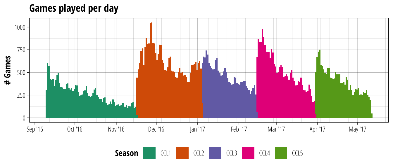
Clearly everyone took a bit of time to come around to the format, with the first season only having an average of 260 games per day, compared with 610, 450, 500 and 400 for the following seasons.
There is also a pretty consistent pattern of an initial burst of activity in the first few weeks which tapers off as the end of a season approaches. There is also an obvious cyclical pattern within each season that most likely results from an increased number of games being played on the weekend. Only the last week of season two runs counter to these trends. Since this time is also around the end of December and start of January, I’m going to assume the everyone got so sick of family over Christmas and needed to recover with a calming match of Blood Bowl.
Because there is such a consistent pattern between seasons, it might be worth seeing how well we can predict the number of games played each day. From the graph above, it seems like the main pattern is an exponential decay, in which the total number of games drops by a percentage of the previous day’s play. So we will model the number of games as: \[\log(n) = \beta_0s_i + \beta_1d + \beta_2w\] where \(n\) is the number of games played in a day, \(s_i\) is the initial number of games for ladder season \(i\), \(d\) is the number of days the season has been running and \(w\) is a true/false term indicating if the day is a weekend. The three \(\beta\) coefficients are what will be estimated in our model and will tell us the relative contribution of \(s_i\), \(d\), and \(w\) to the number of games played in a Champion League season.
games_per_day <- time_data %>%
  group_by(Season, d = lubridate::date(started)) %>%
  summarise(n_games = n()) %>%
  mutate(days_running = d-min(d), is_weekend = lubridate::wday(d, label = T, abbr = T) %in% c("Sat","Sun"))

model = lm(log(n_games) ~ 0 + Season + days_running + is_weekend, data = games_per_day)

games_per_day$predicted = exp(model$fitted.values)

season_plot +
  geom_step(data = games_per_day, aes(x = as.POSIXct(d), y = predicted, group = Season)) +
  labs(subtitle = "With number of games from fitted model")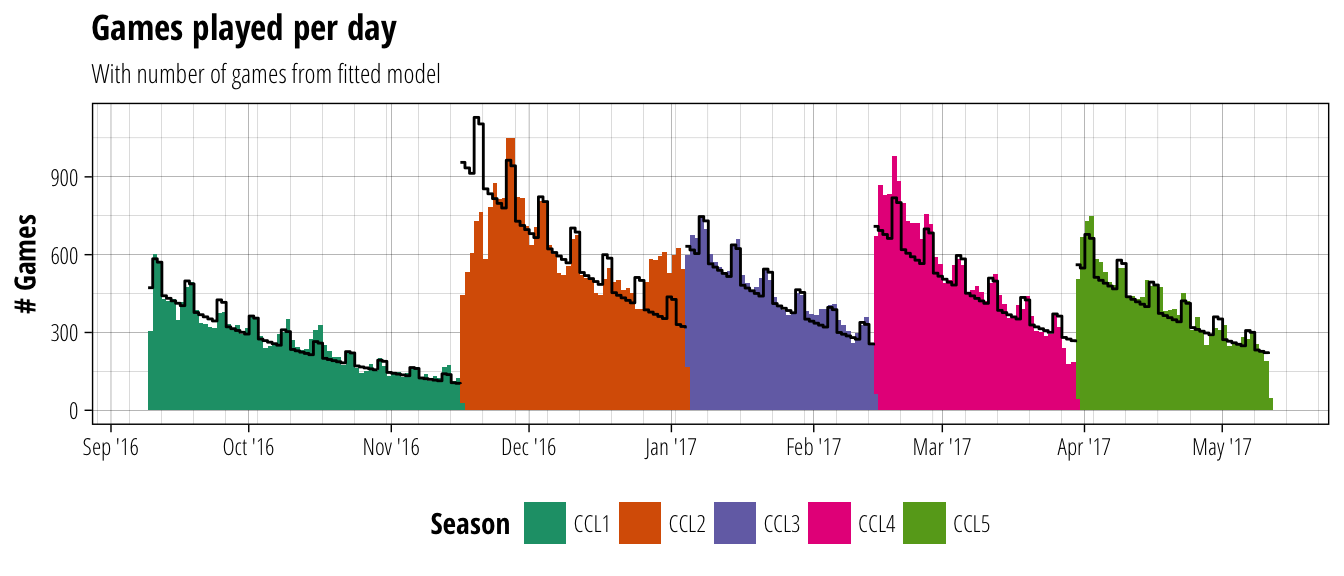
It looks like the fitted model does a good job of tracking the variation in games played, with the exception of the start and end of season 2. So what can this model actually tell us? By converting the estimated coefficients into percentage changes, we find that each day the season runs for sees a drop in games played of 2.23% from the day before (95% confidence interval 2.04–2.42%). If the day is a weekend, however, it is expected that there will be a boost of 26.4% more games played than if it were a weekday (95%CI 18.2–35.2%).
We can also find the most popular time of day to play by looking at how many games start within each hourly window across the course of a season.
time_data %>%
  ggplot(aes(x = hour(started))) +
  geom_histogram(binwidth = 1) +
  scale_x_continuous(NULL, breaks = seq(0,23,by=4), labels = function(b) paste0(b,":00")) +
  guides(fill="none") +
  labs(title = "Games started by hour of day",y = "# Games")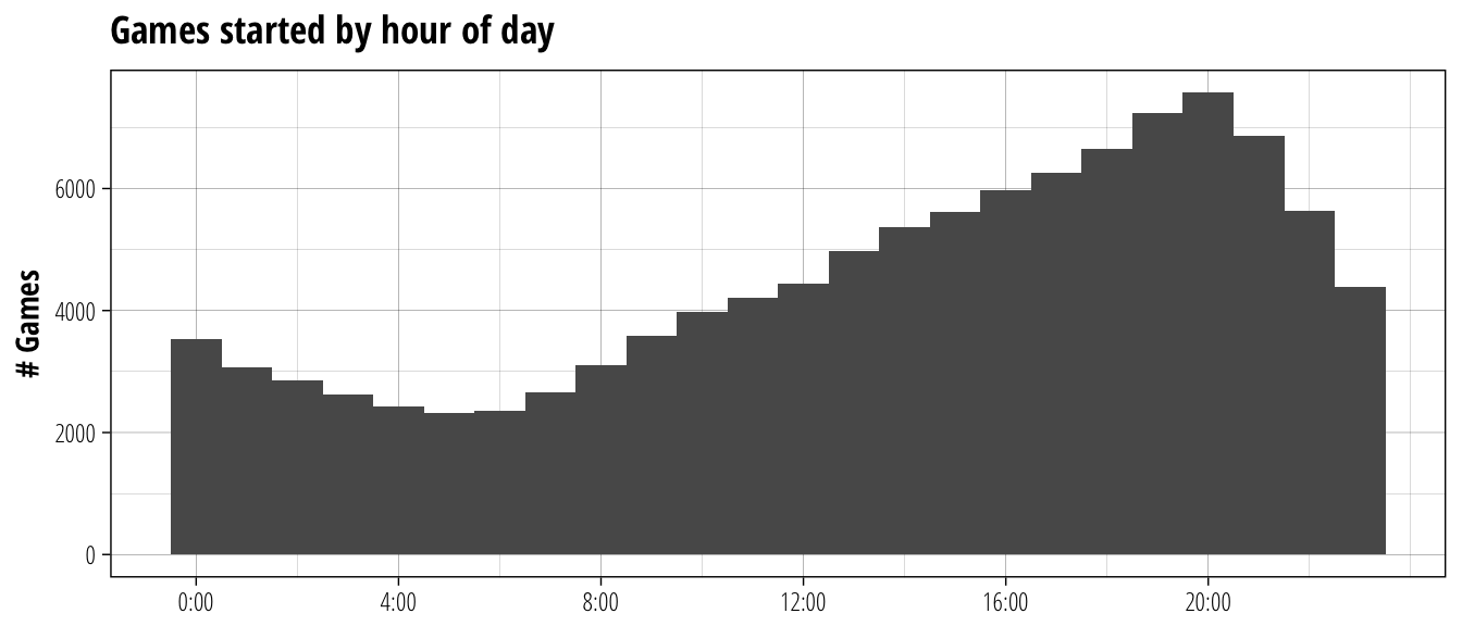
Since Blood Bowl seems to have a very strong European-based community, it’s not that surprising to see that evenings (Paris time) are the busiest time to find a match. For those of us outside that region, I guess we have to either live with the potential matchmaking issues with having fewer people in the queue or find a way to avoid the midnight – 08:00 window where very few games occur.
Just one more game…
The eternal question. It’s getting late, you really should go to bed, but there’s time to squeeze in one last game, right? Let’s look at how long each of the Champion Ladder games took so that next time the question arises, we can be somewhat rational about it.
Obviously whether the game is played to completion will affect how long it takes, so we will need to look at conceded games separately.
game_length <- time_data %>%
  mutate(g_l = difftime(finished, started, units = "mins"), game_completed = home_mvps == 1)

ggplot(game_length, aes(x = g_l, fill = game_completed)) +
  geom_histogram(alpha = 0.8, position = "identity", binwidth = 1) +
  scale_x_continuous(breaks = seq(0, 150, by = 30)) +
  scale_fill_brewer("Completed",palette = "Set1", labels = c("No", "Yes")) +
  labs(title = "How long for a game?", x="Game length (mins)", y = "# Games")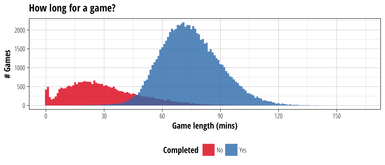
There are a lot more concessions than I was expecting from a format that punishes them pretty heavily. We can also see the difference between inducement screen bugs, which occur in the first few minutes, and the more usual rage quit/pixel hugging concessions, which take at least ten minutes before throwing in the towel. I guess one piece of good news is that if the game gets past 50 minutes, it becomes more likely to run to completion than not.
For completed games, the average game length is 75 minutes, with about 70% of the games finishing between 60 and 90 minutes. The 90 minute mark is a good one to use when thinking about how long you’ll need to commit to a game, because it’s at the 83rd percentile of completed game length. This means that 5/6 games finish before 90 minutes and 1/6 finish later. So when you’re considering if it’s worth spinning for one final game, ask yourself if you would risk a GFI on staying up for more than an hour and a half.
Late starter
If you are the sort of person who doesn’t play the Champion Ladder competitively, but as a way of getting a better quality game, it can be a bit confusing about whether it’s worth starting a team in the last few weeks of a season. Will there be enough fresh teams around that it’s likely to get a balanced match? Or is it all teams with much more development that, while beatable, often aren’t as fun to play against with a new team?
For our purposes, we’ll conservatively define a fresh team as one that has played three or fewer games. Looking at the proportion of fresh teams in the total playing population will give us some idea of whether it’s worth starting fresh later in the season.
#Need to interleave the team names first
interleaved_teams = data_frame(
  team    = c(time_data$home_team, time_data$away_team)[order(rep(1:nrow(time_data), times = 2))],
  started = rep(time_data$started, each = 2),
  Season  = rep(time_data$Season, each = 2)
)

interleaved_teams %>%
  group_by(Season, team) %>%
  mutate(n_games = row_number(), is_fresh = n_games <= 3) %>%
  ggplot(aes(x = started, fill = is_fresh)) +
  geom_histogram(alpha = 0.8, position = "fill", binwidth = as.numeric(lubridate::days(1))) +
  scale_x_datetime(NULL,date_breaks = "2 week", date_labels = "%d/%m", expand = c(0,0)) +
  scale_y_continuous("Proportion",breaks = seq(0, 1, by = 0.1), labels = function(b) paste0(b*100," %"), expand = c(0,0)) +
  scale_fill_brewer("Team type", palette = "Set1", labels = c("Experienced ", "Fresh "), direction = -1) +
  facet_wrap(~Season, scales = "free_x") +
  labs(title = "Proportion of fresh teams in the pool", subtitle = "Fresh = played no more than three games")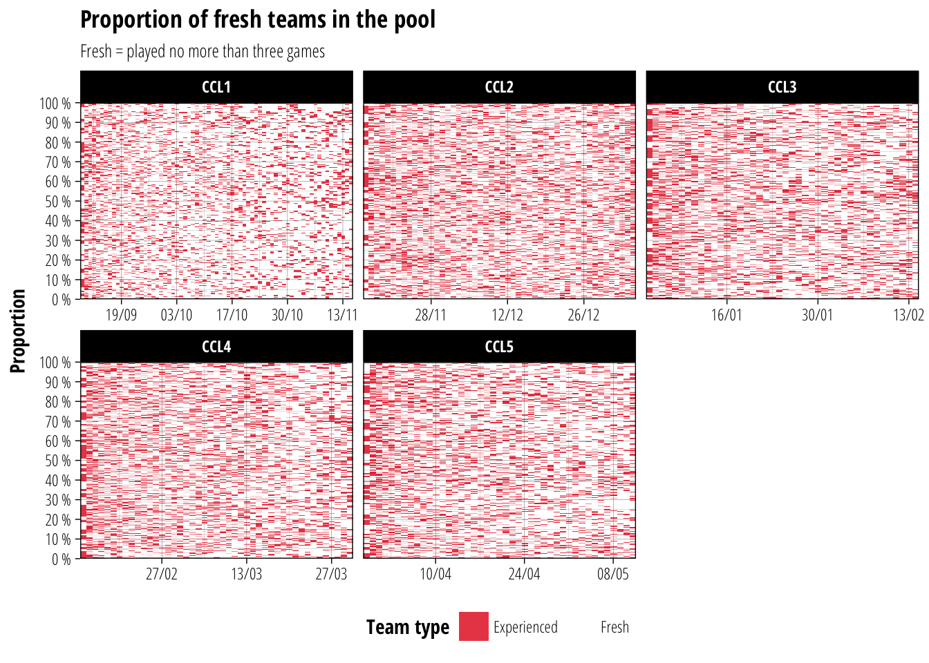
After the initial week where most teams are fresh, it seems to settle into a stable pattern for the remainder of the season. This appears to be consistent across seasons as well, with around one third of the teams playing each day having three or fewer matches.
So despite the total number of games decreasing across the life of a season, there doesn’t seem to be any major compositional change to the type of teams playing. Even in the last few days of the season there are still people starting new teams, so there should always be some viable competition at the TV1000 level.
Share this post
Twitter
Google+
Facebook
Reddit
LinkedIn
StumbleUpon
Email