Prediction process

For each game of the season, we will predict the results based on a few factors:

Post-match updating

Once the result of a game has been predicted, we update a team’s record and TV so that it is ready for the next round. Updating the record is very simple, just add the predicted result of the game. To update the team’s TV to a new value, we will again be making use of the CCL data for equivalent teams.

We originally found that there was a relationship between a team’s pre-game and post-game TV. Specifically, the higher TV a team, the more likely it was to lose TV for the next game. Unsurprisingly, this effect is different for different races with the lower AV teams bouncing around in TV much more than teams with more durable players.

library(nufflytics)

ccl_tv_change %>% 
  ggplot(aes(x = tv, y = tv_change)) +
  geom_hex(bins = 50) +
  facet_wrap(~race) +
  viridis::scale_fill_viridis("Count", trans = "log10") +
  labs(title = "TV gain/loss at different TV levels", subtitle = "Ignoring the first two games of a team's record", x = "TV", y = "Post match TV change")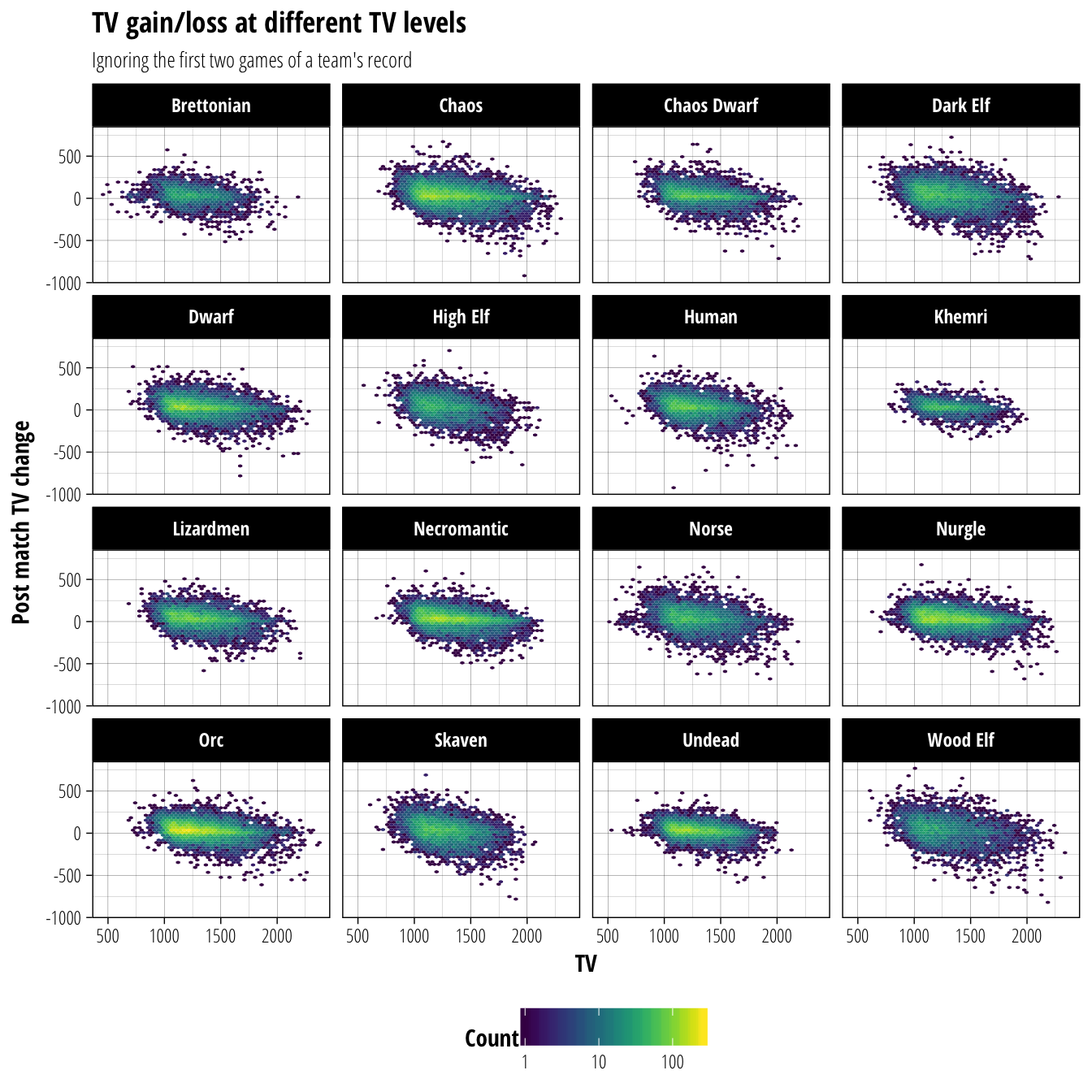

For anyone interested in Blood Bowl analysis in R (probably only me, but who knows!) you will notice that the code block above loads my own work-in-progress package to be used for the season predictions. I’ll be adding other useful functions for Blood Bowl analysis to it as I go, so contact me if you are interested in trying it out.

To update a team’s TV after a match prediction, we will randomly sample from the TV change outcomes for a CCL team of the same race within +/- 20 TV. To limit the impact of outliers on this prediction, we will sample multiple times and use the median to update a team’s TV.

REL Division 1

We are going to start our predictions with REL as they provided the Superbowl winner for season 5 (let’s be honest, they probably don’t have the attention span to read much further anyway). Since it’s the first, I’ll walk through the steps in a bit more detail here and then provide just the predictions for the other leagues.

Data inputs

The inputs we need for running a simulation are pretty basic. First we need some data about the teams in the league (only a few teams shown in this example):

REL_teams <- read_csv(paste0(data_dir, "REL/REL_S6_Div1_teams.csv"))

team_name	race	coach	TV_displayed	TV_extra	wins	draws	losses
Pastry Pests	Skaven	Luminous	1660	100	41	13	10
Men in Tights	Wood Elf	SlightlyBent	1750	90	11	8	12
USS Sulaco (REL Chapter)	Lizardmen	IsenMike	1610	180	30	7	14
Handsome Jacks	Human	VaporGecko	1590	50	19	14	20
Yeti to Party	Norse	SoulOfDragnFire	1720	50	27	6	10
AnimalFarm	Chaos	Saace	1900	0	8	13	19

The TV_displayed column is the team’s TV as shown in game, while TV_extra is the TV that should be added to take a team up to their ‘true’ TV. This included any journeymen the team will require, as well as any players who are unavailable for the first round of the season. The rest of the data should be fairly self-explanatory, with the reminder that spin games have been removed from a team’s record. Perhaps the only other comment to be made from this example is to wonder how REL let a team with an 8-13-19 record survive in their top division. With the fearsome reputation of REL Div1 I would have expected that any team suffering such a record would be broken beyond repair.

The remaining information we need is the schedule for the league, recording the round number, home team and away team for each match:

REL_schedule <- read_csv(paste0(data_dir, "REL/REL_S6_Div1_schedule.csv"))

round	home_team	away_team
1	The Saskatoon Shiners	The Booze Cruise
1	Treat Kune Do	Bad Guys Inc
1	Gloom & Zoom	Necronomics
1	Refrigerator Raiders	Pastry Pests
1	Knights who said Ni	Men in Tights
1	AnimalFarm	USS Sulaco (REL Chapter)

#Takes a while to run (~1 hour for 1000 sims on my machine)
#REL_simulation <- simulate_league(teams = REL_teams, schedule = REL_schedule, weights = list(c(40,30,30)), num_sims = 1000)

#So instead, load the previously completed results
load(paste0(data_dir,"REL/REL_S6_Div1_simulation.Rdata"))

#Rank teams by the number of times they end up on top of the division
rank_teams <- function(sim_results) {
  sim_results %>% 
    group_by(sample) %>% 
    filter(round == max(round)) %>% 
    filter(score == max(score)) %>% 
    group_by(team) %>% 
    summarise(victories = n()) %>%
    mutate(pct = paste0(round(victories/sum(victories)*100, 1),"%")) %>% 
    arrange(desc(victories))
}

#Plot average points gained for each team
plot_results <- function(sim_results, team_rank, title, label_height = 0) {
  sim_results %>% 
    filter(round == max(round)) %>% 
    mutate(team = factor(team, levels = team_rank$team)) %>% 
    #group_by(team) %>% 
    ggplot(aes(x = team, y = score)) +
    stat_summary(fatten = 2, fun.data = function(d) mean_cl_boot(d, conf.int = 0.99)) +
    geom_label(aes(x = team, y = label_height, label = pct), size = 3, data = team_rank) +
    theme(axis.text.x = element_text(angle = 45, hjust = 1, vjust = 1)) +
    labs(title = title, x = "Team", y = "Average score")
}

REL_team_rank <- rank_teams(REL_simulation)

plot_results(REL_simulation, REL_team_rank, "REL Div1 predictions", 10)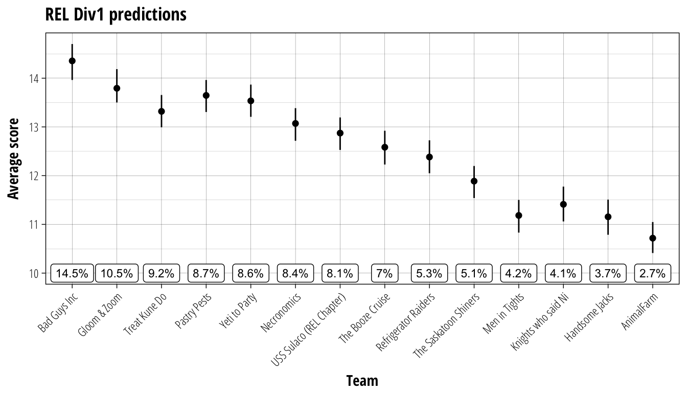

This figure provides a summary of the simulation results for REL Division 1, with the teams ordered left to right by the percentage of simulations in which they finished in first place (displayed just above the name). Also shown is the average end of season points tally for each team, along with a measure of variability.¹ Don’t try to interpret these too strictly, but if the ranges for two teams do not overlap it means we predict that it is likely that the team with the higher average will finish above the other team.

Because Blood Bowl has a significant luck component, you will see that there is often not a lot of difference between teams and that even teams with the lowest average score end up at the top of the table in some simulations. With four playoff spots available for the division, the weight of numbers appear to be backing Bad Guys Inc, Gloom & Zoom, Pastry Pests and Yeti to Party to represent REL Div1 in the big dance. The dark horse of the division would have to be Treat Kune Do, coming out with the third highest percentage of simulations at the top of the table but only the fifth highest average points. With how rapidly a Wood Elf team’s prospects can change based on injury dice, if zuark can protect his players against the meatgrinder of REL Div1 I would not be surprised to see him making an impact in the post-season.

Gman Division 1

With Gman down in numbers for this season, Division 1 loses out on a playoff berth from last season. This makes it just that little bit harder for the top flight Euro teams, with 14 high-quality teams battling it out for only three places in the playoffs. Since you must all be bored of my pointless words by now, let’s just get straight into the predictions. We will be using exactly the same simulation parameters as for REL.

Gman_teams <- read_csv(paste0(data_dir, "Gman/Gman_S6_Div1_teams.csv"))
Gman_schedule <- read_csv(paste0(data_dir, "Gman/Gman_S6_Div1_schedule.csv"))

#Gman_simulation <- simulate_league(teams = Gman_teams, schedule = Gman_schedule, weights = list(c(40,30,30)), num_sims = 1000)
load(paste0(data_dir,"Gman/Gman_S6_Div1_simulation.Rdata"))

Gman_team_rank <- rank_teams(Gman_simulation)

plot_results(Gman_simulation, Gman_team_rank, "Gman Div1 predictions", 10.5)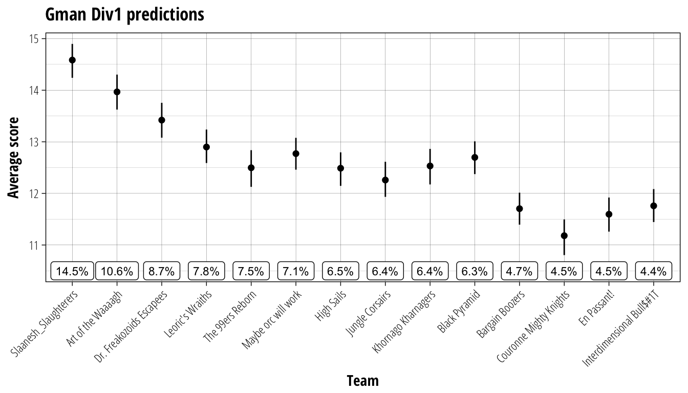

The top of the table for Gman is a little more certain than was seen for REL. The Slaanesh_Slaughterers and Art of the Waaaagh are each predicted to perform significantly better than the rest of the competition and it would be unexpected if they were not title contenders by the final round. The all important third place and the playoff ticket that comes with it is much more contested however. While Dr. Freakozoid’s Escapees are tipped to claim the position, there are many teams snapping at their heels, with Leoric’s Wraiths, Maybe orc will work, and Black Pyramid leading the pack.

Big O Division 1

We now come to the Big O, a league close to my heart. Since there are only three divisions, and I already had the data for Division 2 from my season preview, we are going to run predictions for everything to test how the system performs for teams with different levels of development.

First up we have Division 1. Three playoff spots on offer and all simulation parameters the same as for REL and Gman.

BigOD1_teams <- read_csv(paste0(data_dir, "BigO/BigO_S6_Div1_teams.csv"))
BigOD1_schedule <- read_csv(paste0(data_dir, "BigO/BigO_S6_Div1_schedule.csv"))

#BigOD1_simulation <- simulate_league(teams = BigOD1_teams, schedule = BigOD1_schedule, weights = list(c(40,30,30)), num_sims = 1000)
load(paste0(data_dir,"BigO/BigO_S6_Div1_simulation.Rdata"))

BigOD1_team_rank <- rank_teams(BigOD1_simulation)

plot_results(BigOD1_simulation, BigOD1_team_rank, "BigO Div1 predictions", 10.5)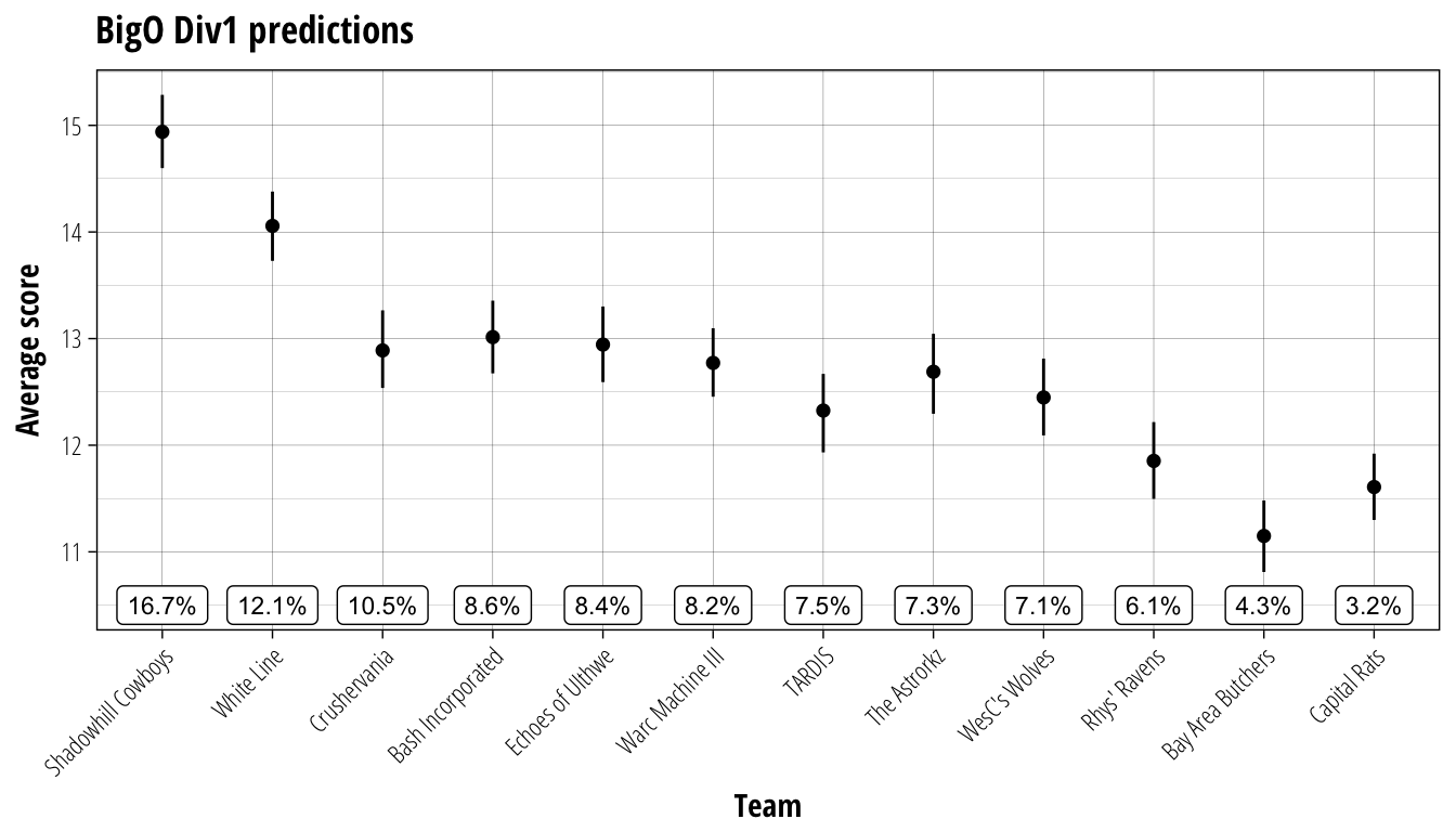

It seems that the prediction algorithm is on the hype train for the Shadowhill Cowboys v White Line rematch, with both teams well ahead of the others. The race for the final playoff spot will be hotly contested however, with seven teams all in the running. A stellar performance to win the Open Invitational suggests that Bash Incorporated may be slightly favoured to claim this prize, however Crushervania, Echoes of Ulthwe, Warc Machine III, TARDIS, The Astrorkz, and WesC’s Wolves are all expected to push hard and make PapaNasty earn his place. Many fans were hoping that the battered and bruised Rhys’ Ravens — pulled out of retirement for one last hurrah — would again bask in the glory of a tilt at the Superbowl. Sadly, the fate of last season’s underdog is predicted to be far more pedestrian with a not-quite-last placing before riding off into the sunset.

BigO Division 2

In Division 2, most of the teams have only a single season of development. The only exceptions here are Cold Coast Cut-throats, who have dropped down after a disappointing last season in Division 1, and Old Hobart Honeybadgers and Catastrophy, who entered Division 3 partway through last season. Since the teams are still relatively new, we will reduce the weighting given to the team’s individual record when predicting results. Instead, we will base our predictions 60% on CCL matchups at the same TV difference, and 20% on each team’s record.

#Allow slightly more weight for team TV & development since these teams have almost all had only 1 season.
BigOD2_teams <- read_csv(paste0(data_dir, "BigO/BigO_S6_Div2_teams.csv"))
BigOD2_schedule <- read_csv(paste0(data_dir, "BigO/BigO_S6_Div2_schedule.csv"))

#BigOD2_simulation <- simulate_league(teams = BigOD2_teams, schedule = BigOD2_schedule, weights = list(c(60,20,20)), num_sims = 1000)
load(paste0(data_dir,"BigO/BigO_S6_Div2_simulation.Rdata"))

BigOD2_team_rank <- rank_teams(BigOD2_simulation)

plot_results(BigOD2_simulation, BigOD2_team_rank, "BigO Div2 predictions", 9.5)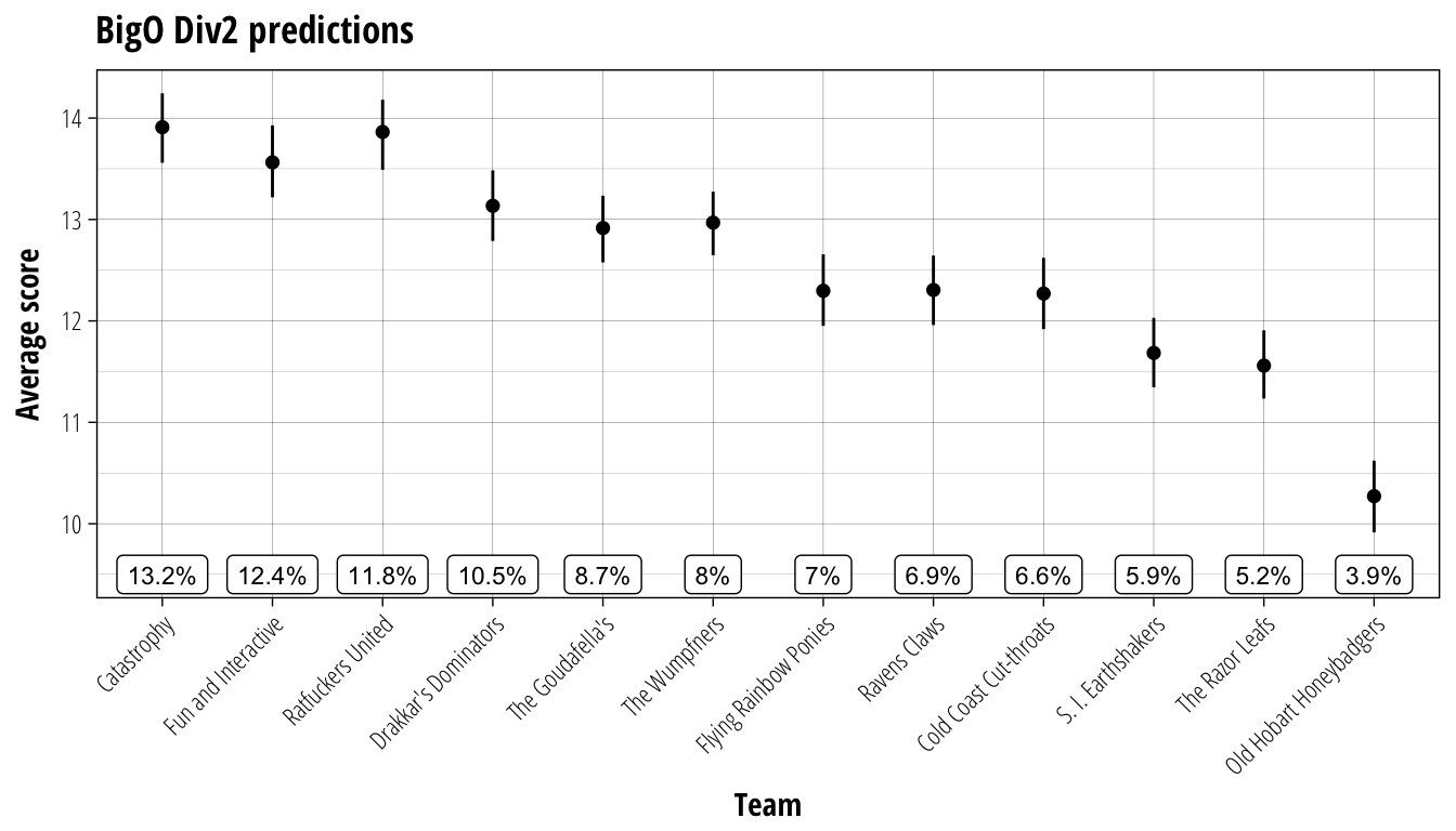

Perhaps a quirk of the algorithm, but Catastrophy is predicted to play a blinder in their first full season in REBBL. Running 4-0-0 to finish out Season 5, the team has certainly made their mark in a short space of time. If they can carry that form through to the new season they will certainly be a force to be reckoned with.

While I would feel a sense of professional satisfaction were Catastrophy to clean up, my head tells me that the next two teams are the ones more likely to be carrying the hopes and dreams of Big O Division 2 in a drive towards the Superbowl. Both Fun and Interactive and Ratfuckers United were solid performers last season and only narrowly missed out on promotion to Division 1. Interestingly, the international contingent are all predicted to bring a bit of excitement to the Big O, with Drakkar’s Dominators, The Goudafella’s, and The Wumpfners all vying for a high position on the leaderboard.

BigO Division 3

As a division of fresh teams I am not expecting to be able to predict much, but with only a single playoff spot we might be able to see who are the main contenders. To compensate for the fact that we have very litle prior information about these teams we will make a few changes to the simulation process.

The first change is to allow spin games to count towards a team’s record when predicting results. They might not provide good information but they are the best we have for a new division. We will also adjust the weighting system to one that changes across the season. For round one we will be predicting results 100% from the CCL data and this will slowly shift over the course of the season to be 60%-20%-20% in the final round in line with the settings used for Division 2. The idea behind this change is that as more games are played we will have a better understanding of the team’s performance, and therefore can take greater notice of that record in predicting results. The final change will be to adjust the schedule to remove bye weeks. While these will probably have a big impact on the division with the chance to refresh players and get some much needed cash their effects are currently too difficult to model and so will just be ignored in our simulations.

Will this be able to provide useful predictions? I have absolutely no idea but am looking forward to finding out.

BigOD3_teams <- read_csv(paste0(data_dir, "BigO/BigO_S6_Div3_teams.csv")) 

#Remove admin teams from schedule
BigOD3_schedule <- read_csv(paste0(data_dir, "BigO/BigO_S6_Div3_schedule.csv")) %>% 
  filter(!grepl("Admin",home_team), !grepl("Admin",away_team))

#Shift weights from (100,0,0) to (50,25,25) over the season
D3_weights <- map(seq(100,60, length.out = max(BigOD3_schedule$round)), ~c(., (100-.)/2, (100-.)/2))

#BigOD3_simulation <- simulate_league(teams = BigOD3_teams, schedule = BigOD3_schedule, weights = D3_weights, num_sims = 1000)
load(paste0(data_dir,"BigO/BigO_S6_Div3_simulation.Rdata"))

BigOD3_team_rank <- rank_teams(BigOD3_simulation)

plot_results(BigOD3_simulation, BigOD3_team_rank, "BigO Div3 predictions", 9)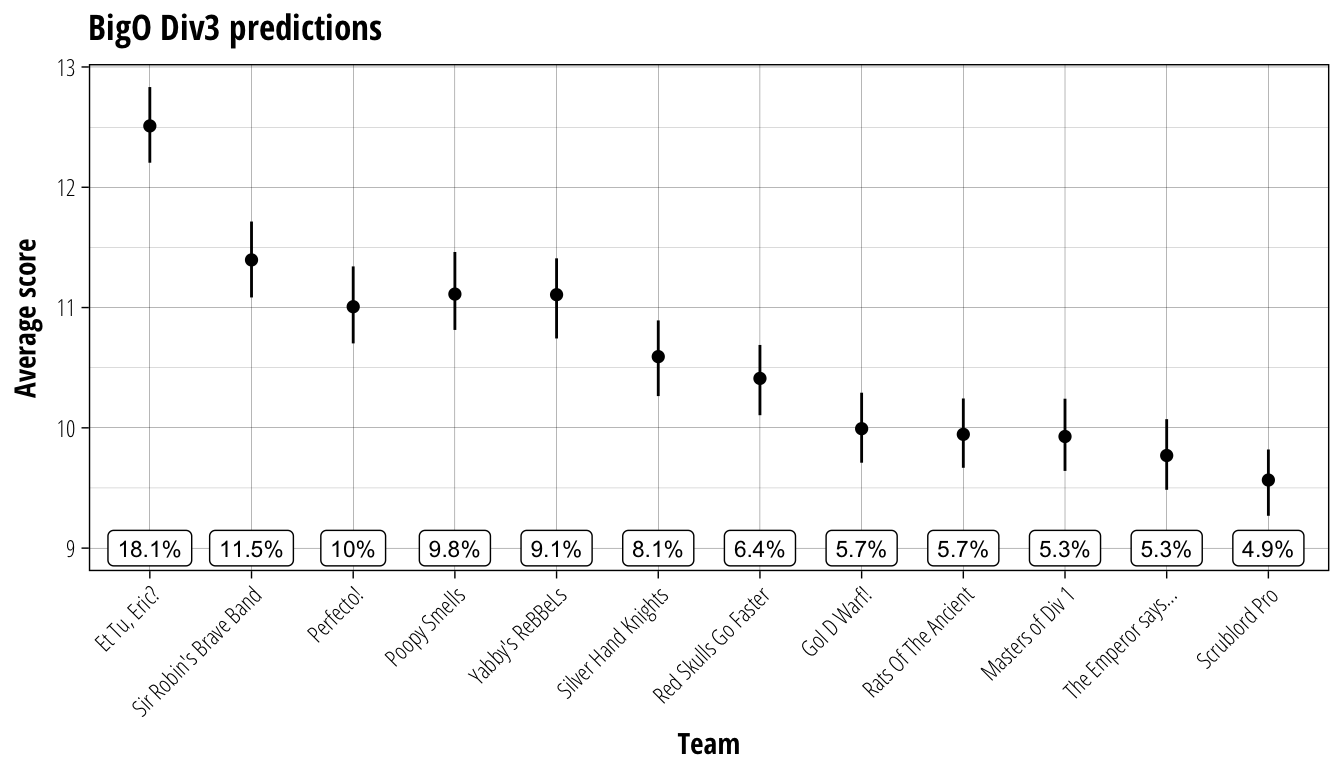

Despite all teams starting off on a relatively even footing we can see that a clear winner is predicted, with Et Tu, Eric? the strong favourite to come out on top. This is a very interesting prediction to make as the Khemri team has neither the highest TV nor the best spin record heading in to the first round. The main challengers would appear to be Sir Robin’s Brave Band, Perfecto!, Poopy Smells, and Yabby’s ReBBeLs with the rest of the division all clustered behind them. I’ll be keeping a very close eye on the results of this division as they come out and cheering strongly for The Peacock as an ambassador for the work of the Institute.